8. Examples

8.1. Focus field calculations

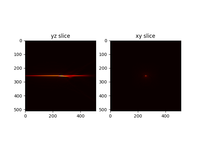
#The following snippet calculates the 3d focus field (PSF) of a simple beam with NA = 0.8 (both scalar and vectorial):

from biobeam import focus_field_beam
N = 256
dx = 0.02

# return the intensity
u = focus_field_beam(shape = (N,)*3,
               units = (dx,)*3,
               NA = 0.8, n0 = 1.33)

# return all the complex vector components
u2, ex,ey,ez = focus_field_beam(shape = (N,)*3,
               units = (dx,)*3,
       NA = 0.8,
               n0 = 1.33,
               return_all_fields = True)

# vizualize
import matplotlib.pyplot as plt
plt.subplot(1,2,1)
plt.imshow(u[...,N//2].T, cmap = "hot")
plt.title("yz slice")
plt.subplot(1,2,2)
plt.imshow(u[N//2,...], cmap = "hot")
plt.title("xy slice")
plt.show()

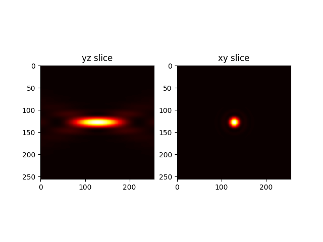
8.2. Plane wave scattered by sphere

from biobeam import Bpm3d
import numpy as np

# create the refractive index difference
N = 512
dx = 0.1
r = 4
x = dx*(np.arange(N)-N//2)
Z, Y, X = np.meshgrid(x,x,x,indexing = "ij")
R = np.sqrt(X**2+Y**2+Z**2)
dn = 0.05*(R<2.)

# create the computational geometry
m = Bpm3d(dn = dn, units = (dx,)*3, lam = 0.5)

# propagate a plane wave and return the intensity
u = m._propagate(return_comp = "intens")

# vizualize
import matplotlib.pyplot as plt
plt.subplot(1,2,1)
plt.imshow(u[...,N//2], cmap = "hot")
plt.title("yz slice")
plt.subplot(1,2,2)
plt.imshow(u[N//2,...], cmap = "hot")
plt.title("xy slice")
plt.show()

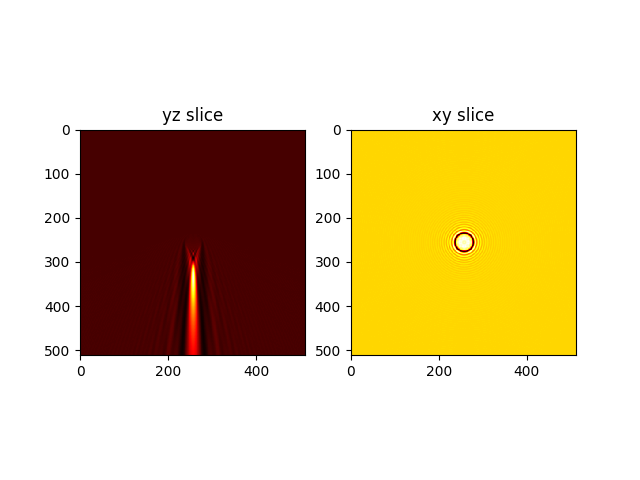
8.3. Cylindrical light sheet through sphere

from biobeam import Bpm3d
# create the refractive index difference
N = 512
dx = 0.1
r = 4
x = dx*(np.arange(N)-N//2)
Z, Y, X = np.meshgrid(x,x,x,indexing = "ij")
R = np.sqrt(X**2+(Y-.9*r)**2+Z**2)
dn = 0.05*(R<r)

# create the computational geometry
m = Bpm3d(dn = dn, units = (dx,)*3, lam = 0.5)

# propagate a plane wave and return the intensity
u = m._propagate(u0 = m.u0_cylindrical(NA = .2), return_comp = "intens")

# vizualize
import matplotlib.pyplot as plt
plt.subplot(1,2,1)
plt.imshow(u[...,N//2].T,cmap = "hot")
plt.title("yz slice")
plt.subplot(1,2,2)
plt.imshow(u[N//2,...], cmap = "hot")
plt.title("xy slice")

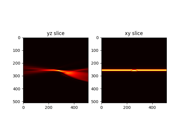
8.4. Single Bessel beam through sphere

from biobeam import Bpm3d
# create the refractive index difference
N = 512
dx = 0.1
r = 4
x = dx*(np.arange(N)-N//2)
Z, Y, X = np.meshgrid(x,x,x,indexing = "ij")
R = np.sqrt(X**2+(Y-.9*r)**2+Z**2)
dn = 0.05*(R<r)

# create the computational geometry
m = Bpm3d(dn = dn, units = (dx,)*3, lam = 0.5)

# propagate a plane wave and return the intensity
u = m._propagate(u0 = m.u0_beam(NA = (0.5,0.52)), return_comp = "intens")

# vizualize
import matplotlib.pyplot as plt
plt.subplot(1,2,1)
plt.imshow(u[...,N//2].T,cmap = "hot")
plt.title("yz slice")
plt.subplot(1,2,2)
plt.imshow(u[N//2,...], cmap = "hot")
plt.title("xy slice")